In this task we are going to extend our pathfinding algorithm and show how we can compute the distances from a given node \(s\) to every other node.
In this context, the distance between two nodes is defined as the minimum number of edges in any path between them. Later, we will consider weights on the edges and see how to compute shortest paths, that is, paths such that the sum of the weights of the edges is as small as possible. You can think of this case as a specification of the general shortest path problem when all edge weights are equal to \(1\).
We will see that the pathfinding algorithm already has everything that we need in order to be able to compute the distances. To see this, we will execute the algorithm again on the same graph but drawing it in a way that the nodes are organized by distance layers. That is one layer for nodes at distance 0, one for nodes at distance 1, and so on.
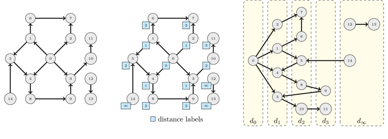
Take the previous graph and label each node with its distance from node \(s = 0\) and redraw it by placing the nodes that have the same distance on the same layer as show in the following figure.

On the left you can see the original graph, in the middle the same graph where each node is labeled with its distance from \(s\) and, on the right, the same graph but with nodes grouped by distance layers. The set \(d_x\) denotes the nodes at distance \(x\) from \(s\). Nodes that are unreachable are put into a set that denoted by \(d_\infty\) and we usually define their distance to be \(+\infty\).
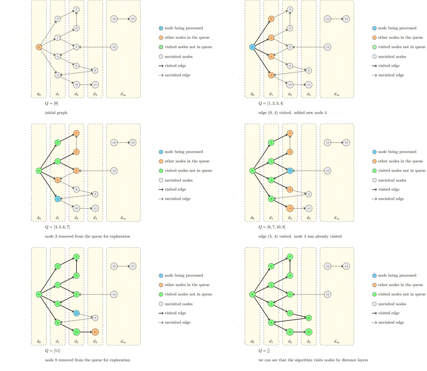
Now we execute again the algorithm but drawing the graph with distance layers:

What do you observe?
The algorithms visits the node layer by layer! The source node :math`s` is obviously at distance \(0\). Every time a node puts a new node into the queue, the node that was added belongs to the next layer. This means that its distance from \(s\) is equal to 1 plus the distance of the node that put it into the queue.
Denote by \(distance(u)\) the distance from \(s\) to \(u\). Then we can write that if node \(u\) adds node \(v\) into the queue it holds
In terms of code we can simply replace the visited set by a distance array that keeps the distances initialized to \(+\infty\). In this setting, a node has been visited if and only if its distance is finite. When a node is added to the queue, instead of marking it as visited we will set his distance to one more than the node that is being processed. Infinity is represented by Integer.MAX_VALUE.
static int[] distances(LinkedList<Integer>[] g, int s) {
    // initialize the queue and visited set
    Queue<Integer> Q = new LinkedList<>();
    Q.add(s);
    int[] distance = new int[g.length];
    Arrays.fill(distance, Integer.MAX_VALUE);
    distance[s] = 0;
    // loop while there are nodes in the queue to process
    while(!Q.isEmpty()) {
        int u = Q.poll();
        // we are now processing node u
        for(int v : g[u]) {
            // visit edge (u, v)
            if(distance[v] == Integer.MAX_VALUE) {
                // node v has not yet been visited, add it
                Q.add(v);
                // set the distance of v
                distance[v] = 1 + distance[u];
            }
        }
    }
    // return the distances from s
    return distance;
}
This algorithm is commonly know as Breadth-first Search (BFS). The reason for this name is because of the fact that it explores all nodes at distance \(d\) before exploring nodes at distance \(d + 1\). Its runtime is \(O(V + E)\) where \(V\) is the number of nodes in the graph and \(E\) is the number of edges. An easy way to see why this is the case is to count how many operations are performed at each node.
Each node is expanded once, when it is removed from the queue. Therefore, in the worst case the while loop is executed \(V(G)\) times (one time for each node). Each iteration of the while loop costs \(1 + g[u].size()\). Thus the total run time is
 INGInious