 INGInious
Dijkstra's algorithm is an algorithm to compute shortest paths in graphs with non-negative edge weights. Denote by \(w(u, v)\) the weight of edge \((u, v)\).
As BFS, we will design the algorithm to receive a source node \(s\) as input and compute the shortest path distances to each other node in the graph.
Let \(dist\) be an array such that \(dist[v]\) is equal to the shortest path distance between node \(s\) and node \(v\). The idea of Dijkstra's algorithm is to keep a set of nodes \(S\) for which we know the value of \(dist\) and grow it until \(S = V\).
Since there are no negative edge weights, we know that \(dist[s] = 0\). This means that we can initialize \(S = \{s \}\). For the other nodes, we initially set \(dist[v] = \infty\).
Given the set \(S\), how can we find a new node to add to it and its distance?
We will consider all edges that go from a node in \(S\) to a node outside of \(S\). From all such edges, we will pick an edge \((u, v)\) such that \(dist[u] + w(u, v)\) is minimum. Then, it is not hard to see that, \(dist[v] = dist[u] + w(u, v)\).
To convince yourself that this is indeed the case, imagine that there is a better way of reaching \(v\). Since \(s \in S\) and :math`v notin S`, this alternative path must at some point exit the set \(S\). Suppose that it does to by an edge \((x, y)\) other than \((u, v)\). The following figure illustrates the situation:
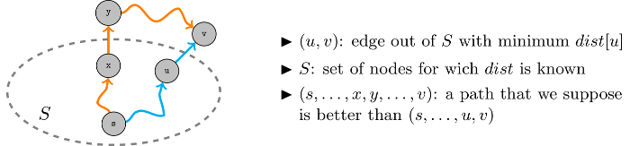
Then, the path (shown in orange) will have the form \((s, \ldots, x, y, \ldots, v)\). Its cost will be
where
- \(dist[x]\) is the cost of reaching \(x\) from \(s\)
- \(w(x, y)\) is the cost of edge \((x, y)\)
- \(cost(y, v)\) is the cost of the path from \(y\) to \(v\)
On the other hand, the blue path has cost:
And we must have
because we selected \(u\) such that \(dist[u] + w(u, v) \leq dist[x] + w(x, y)\) and we know that, since the edge weights are non-negative, \(cost(x, y) \geq 0\).
After this discussion it should be quite straightforward for you implement Dijkstra's algorithm. The high level ideas is the following:
- Initialize \(dist[s] = 0\) and \(dist[v] = \infty\) for each \(v \neq s\)
- Set \(S = \{s\}\)
- While \(S \neq V\), pick \((u, v) \in E\) such that \(u \in S, v \notin S\) and \(dist[u] + w(u, v)\) is minimum and set \(dist[v] = dist[u] + w(u, v)\).
Now the only question is how fast can we perform the edge selection in step 3. The naive way of doing so is to simply loop over each node \(u \in S\) and each edge out of \(u\) to check the condition and get the minimum. This would cost \(O(|E|)\) making the algorithm run in \(O(|V| |E|)\) since there are \(|V|\) iterations.
A more efficient alternative is to use a priority queue. A priority queue enables to maintain a queue of ordered elements and retrieve the minimal element in the order efficiently. In our context, the elements will be the edges sorted by their value of \(dist[u] + w(u, v)\).
The Java code doing this is given below. Note that we do not need to explicitly keep track of the set \(S\). In the way the code is written this set is always equal to the set of nodes such that \(dist[u] \neq \infty\).
// class used to represent edges
static class Edge {

    public int orig, dest, cost;

    public Edge(int orig, int dest, int cost) {
        this.orig = orig;
        this.dest = dest;
        this.cost = cost;
    }

}

// class used to compare edges in the priority queue
static class EdgeCmp implements Comparator<Edge> {

    private int[] dist;

    public EdgeCmp(int[] dist) {
        this.dist = dist;
    }

    public int compare(Edge e1, Edge e2) {
        double v1 = dist[e1.orig] + e1.cost;
        double v2 = dist[e2.orig] + e2.cost;
        return Double.compare(v1, v2);
    }

}

static int[] disjktra(LinkedList<Edge>[] g, int s) {
    // initialize distances
    int[] dist = new int[g.length];
    Arrays.fill(dist, Integer.MAX_VALUE);
    dist[s] = 0;
    // initialize PQ
    PriorityQueue<Edge> Q = new PriorityQueue<>(new EdgeCmp(dist));
    for(Edge e : g[s]) Q.add(e);
    while(!Q.isEmpty()) {
        Edge mine = Q.poll();
        // check whether the edge goes out of S
        if(dist[mine.dest] == Integer.MAX_VALUE) {
            dist[mine.dest] = dist[mine.orig] + mine.cost;
            for(Edge e : g[mine.dest]) {
                Q.add(e);
            }
        }
    }
    return dist;
}
The runtime of this algorithm is \(O(|E| \log(|V|))\) since each edge will be at most one time in the queue and the priority queue poll and add operations are performed in logarithmic time with respect to the size of the queue. The maximum size of the queue is \(|E|\) so the maximum runtime of a queue operation is \(O(\log(|E|)) = O(\log(|V|^2)) = O(\log(|V|))\).
For you algorithmic culture, it is possible to implement Dijkstra's algorithm using a Fibonacci Heap instead of a priority queue reducing the runtime to \(O(|E| + |V| log|V|)\) but this has little to no use in competitive programming.