 INGInious
In this task we are going to learn how to compute the strongly connected components (SCC's) of a directed graph.
A graph is said to be strongly connected if there exists at least one path between any pair of nodes in that subset.
The strongly connected components of a graph are the maximal strongly connected subgraphs of that graph.
Example:
The following image shows a graph with 4 SCC's. The nodes on the same SCC are colored with the same color.
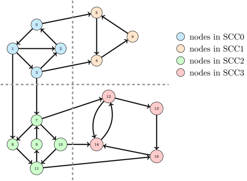
Let's try to get some intuition on how we could compute these SCC's.
Imagine that we start a DFS at any red node, say 13. Then the set of nodes that will be visited is exactly the set of red nodes and no other. So, in this case, we are lucky to visit exactly a SCC of the graph. If we mark the visited nodes as visited and then start from any green node, say 11, we will visit only the green nodes and thus find a new SCC. However, if after that we select a blue node, we will visit all the blue nodes together with the yellow nodes failing to find a new SCC. To avoid this problem we should have first done a DFS from a yellow node and only after that from a blue node.
The following animation illustrates this.
This suggest that as long as we select a good order to perform DFS's, the set of nodes visited in each DFS will correspond to a SCC.
This is actually quite natural as we are going to see now. Observe that the SCC's form a directed acyclic graph that we will refer to as SCC-DAG. By this, we mean that we fuse each SCC into a single node and connect two fused nodes if they contain originally connected nodes (we remove parallel edges).
Example:
The SCC-DAG corresponding to the previous graph is the following:
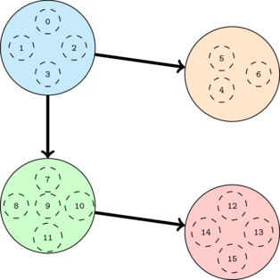
The SCC-DAG must be acyclic because, by definition, the SCC's are maximal strongly connected subgraph. If the SCC-DAG contained a cycle, all the nodes in the corresponding SCC's would have been in the same SCC in the original graph to begin with. Thus contradicting the fact that they resulted in distinct nodes in the condensed graph.
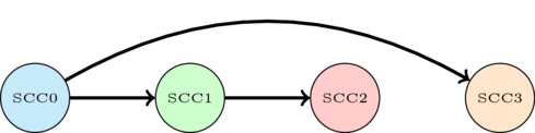
By being acyclic it must have a topological order. This tells us exactly the order in which we should call DFS so that each DFS yields exactly one strongly connected component. We should do it from the last to the first SCC in a topological order of the SCC-DAG, that is, in the reverse order of the SCC-DAG topological order.
Example:
One possible topological order is shown. This tells us that we need to process the red nodes before the green ones, the green ones before the blue ones and the yellow nodes before the blue ones.
Ok, so now we have an idea of what to do. It remains to see how we can do it. So far this idea seems to require us to know the SCC's in the first place... But we are going to see that we can actually very easily compute something close enough to this order with a single DFS.
We saw before that DFS can be used to compute a topological order of a DAG. However what happens when we feed the algorithm a graph that is not a DAG? Obviously it cannot output a topological order since no such order can exist. Let us see what happens by executing it on the same example.
The order, colored with respect to the SCC's, computed by this algorithm is the following:

Observe that if we traverse the order from left to right we do not obtain all the nodes from each SCC grouped together and in order. However, if we write down the order in which the colors appear, this order matches the topological order of the SCC-DAG.
In general it could have been a different order but it will always be a valid topological order of the SCC-DAG (for example, blue, yellow, green red).
The reason why this is true in general is that if a SCC \(C\) is reachable from a node \(u\) then if we call dfsVisit(u), \(u\) will be closed after all nodes from \(C\).
Therefore node \(u\) will come before all nodes in \(C\) in the toposort array. This is a consequence of the more general behaviour of DFS: when we call dfsVisit(u), all nodes reachable from \(u\) will be closed before \(u\).
We almost have what we want! Recall that we saw above that a good order in which to perform DFS would be the reverse of the topological order of the SCC-DAG. We already know how to compute the real order, how about the reverse?
Notice from the example above that just reversing the order is not what we want, the first node would still be a blue node. The reverse order can be obtained by reversing every each of the input graph before computing the toposort array! This works because:
- The SCC remains the same under edge reversal;
- The edges connecting the SCC's are reversed so a topological order of the reverse SCC-DAG must be a reverse topological order of the original SCC-DAG.
The following animation shows the execution of the same algorithm as before but on the reversed graph:
The order that we obtain this time is the following:

As we can see, this time we have a good order to compute the strongly connected components. If we look through the nodes in this order, call DFS on nodes if they are not visited, each DFS call will compute a strongly connected component.
Now that we have all the right ideas, it is quite straightforward to write the code. The high level sketch is the following:
- Compute the reverse graph \(gr\)
- Call toposort on gr obtaining the \(toposort\) array
- Loop over the nodes in order of the toposort array and call
dfsVisiton the original graph \(g\), if the node has not yet been visited, label all the nodes v visited as belonging to the same SCC.
static final int UNV = -1;
// scc will contain the scc label of the nodes
// scc[i] = scc[j] iff i, j are on the same scc
static int[] scc;
static int[] toposort; // toposort will have the node indexes in topological order
static int toposortIndex; // to keep track where to put the next node
static int nbScc; // will contain the number of scc's in the end

@SuppressWarnings("unchecked")
static LinkedList<Integer>[] transpose(LinkedList<Integer>[] g) {
    LinkedList<Integer>[] gt = new LinkedList[g.length];
    for(int i = 0; i < g.length; i++) {
        gt[i] = new LinkedList<>();
    }
    for(int i = 0; i < g.length; i++) {
        for(int j : g[i]) {
            gt[j].add(i);
        }
    }
    return gt;
}

static int[] scc(LinkedList<Integer>[] g) {
    // compute the reverse graph
    LinkedList<Integer>[] gt = transpose(g);
    // get the order
    int[] order = toposort(gt);
    // reset dfs data to visit the SCC's
    initDFS(g);
    // initialize the SCC label, nodes with same label are on the same SCC
    int sccLabel = 0;
    // loop over the nodes in order to visit the SCC's
    for(int u : order) if(scc[u] == UNV) {
        dfsVisit(g, u, sccLabel++);
    }
    nbScc = sccLabel;
    return Arrays.copyOf(scc, scc.length);
}

static void initDFS(LinkedList<Integer>[] g) {
    toposort = new int[g.length];
    toposortIndex = g.length - 1;
    scc = new int[g.length];
    Arrays.fill(scc, UNV);
}

static int[] toposort(LinkedList<Integer>[] g) {
    initDFS(g);
    for(int u = 0; u < g.length; u++) if(scc[u] == UNV) {
        dfsVisit(g, u, 0);
    }
    return Arrays.copyOf(toposort, toposort.length);
}

static void dfsVisit(LinkedList<Integer>[] g, int u, int sccLabel) {
    scc[u] = sccLabel;
    for(int v : g[u]) if(scc[v] == UNV) {
        dfsVisit(g, v, sccLabel);
    }
    toposort[toposortIndex--] = u;
}
To make the implementation shorter we reuse the same data and dropped the unnecessary one. We use the dfsVisit both to compute the topological order and to visit the components afterwards. The scc array serves two purposes: in the first time it is used simply to mark nodes as visited when we are computing the topological order. In the second time we use it to label all visited nodes with the index of the SCC (starting from 1) so that two nodes will have the same label if they are on the same connected component.
Note that in the second execution the toposort array is still update but we don't care about its content, it is just so that we can reuse the same code for the two tasks. So there is a slight loss in semantics on the code but we believe that it is worth the length gain in this case.
Also, note that once we have the topological order, the way each component is visited does not matter. Here we did a DFS because we already have the code but any graph exploration algorithm would do, like a BFS for example.
Important thing to remember:
If you call a toposort on a directed graph, the order you obtain is either a topological order if the graph is acyclic or the nodes will be ordered so that the first occurrence of a node from each SCC appears in a topological order of SCC-DAG.
This is what we saw when we called toposort on the first graph. We obtained:
The first occurrence of each color (blue, green, red, yellow) respects a topological order of SCC-DAG. The colors mix at the end but the first occurrences of each of them respect the order.
This is useful because it allows to find a root for the SCC-DAG, that is, a node that can reach everyone else (provided that such a node exists) without computing the contracted graph.