 INGInious
In this task we are going to learn how to compute the maximum flow between two nodes in a graph. In the maximum flow problem each edge has a capacity and we aim to send the maximum amount of flow (information) between a source node \(s\) and a sink node \(t\) in a graph without exceeding the capacity of any edge.
Example:
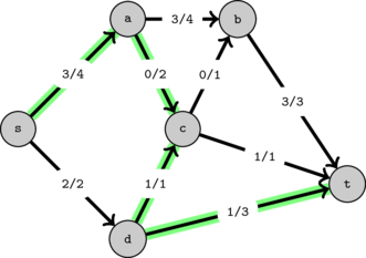
In the following graph, we can send a total of 6 units of flow as shown. The numbers on the edges represent the edge capacities.
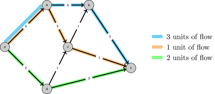
In this example all the edges leaving the source are saturated (have no capacity remaining). Thus we know that must be the maximum flow as we would never be able to send more than this.
By looking at such an example it seems that we can compute the maximum flow simply by finding paths from \(s\) to \(t\) and pushing as much as we can each time. As we will see, this is a little too greedy to work so we will need to refine the idea a bit in order for it to work.
Example:
Consider the same graph but pushing flow on a different set of paths. Every time we find a path from \(s\) to \(t\) we increment the total flow by the minimum capacity edge on that path. We label each edge with \(f / c\) where \(f\) is the flow currently passing on that edge and \(c\) is its capacity.
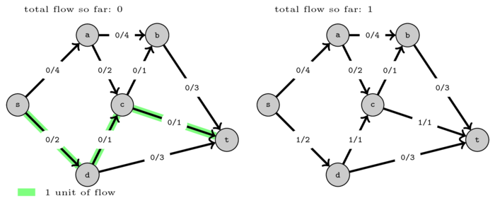
The first path found was \((s,d,c,t)\) and we could push 1 unit of flow.
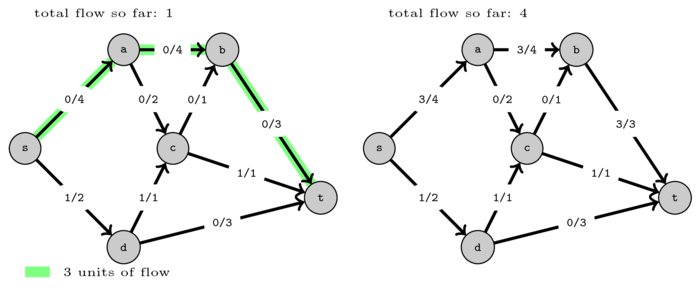
Then we found path \((s,a,b,t)\) and pushed 3 units of flow.
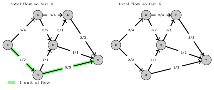
After that we found path \((s,d,t)\) and pushed one more unit of flow. Now there are no more paths from \(s\) to \(t\) with positive capacity in the graph so we cannot push more flow.
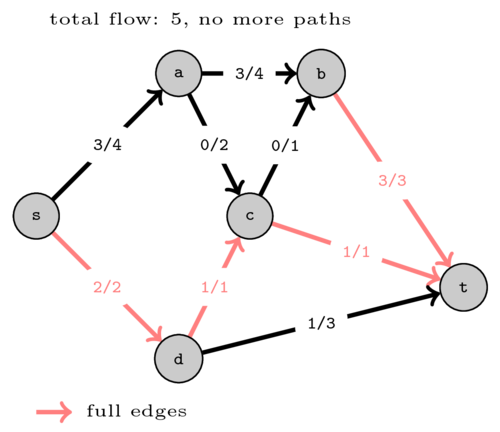
As you can see, we were only able to push a total of 5 units of flow. However on the first example we saw that the maximum flow is 6. This shows that simply finding paths with positive capacity and pushing flow does yield an optimal solution.
This shows that the order in which the paths are selected is important. However, in order to solve the problem, we are not going to develop an algorithm that finds a good order. Rather, we will find a clever way so that we can reroute some of the flow that we are already sending in order to accommodate new flows.
Let's look at the final flow that we obtained before and try to understand what we can change in order to send one more unit of flow.
One way to do that is to first take one unit of flow on \((d, c, t)\) and redirect it to \((d, t)\) as shown in the following figure:
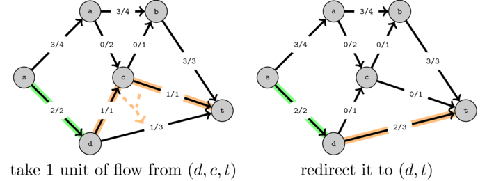
This will free one new unit over path \((s, a, c, t)\):
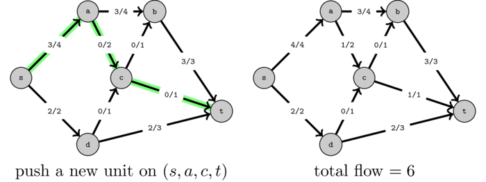
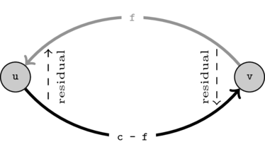
But how can we find this change? It turns out that a simple pathfinding algorithm can achieve it. If you think about it, the two operations that we performed, the redirection plus pushing a new unit of flow, is the same as if we had pushed one unit of flow on the following "path":
This is not really a path as edge \((d, c)\) is traversed in the opposite direction. However if we defined that when we push flow on an edge, if the edge direction is correct then we increase the flow and when the direction is reversed, we decrease the flow, the two operations achieve the same exact flow.

The intuition behind this is that the part of the path until we cross an edge in the reverse direction corresponds to the new path on which we will push flow and the part of the path after the edge in reverse direction corresponds to where we redirect the flow.
This is just a high level intuition as in practice the path could cross several edges in the reverse direction but the idea remains the same.
So how do we implement all this?
For every edge in the input graph, we will create a residual edge with the reverse direction initially with capacity \(0\). Then whenever we push flow \(f\) on one edge \(e\), we decrease the capacity of \(e\) by \(f\) and increase the capacity of \(residual(e)\) by \(f\). This will allow us to find paths that traverse edges in reverse direction allowing us to redirect the flow passing on it towards another path. We call this modified graph the residual graph.
The following figure illustrates this.
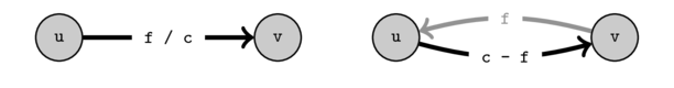
On the left you can see one edge with capacity \(c\) with a flow \(f\) traversing it. On the residual graph this will correspond to an edge with capacity \(c - f\) and one residual edge (in gray) in the reverse direction with capacity \(f\) meaning that we can redirect up to \(f\) units of flow.
Example:
Let's look at the residual network corresponding to the above graph where we were only able to push \(5\) units of flow. We will draw the residual edges in gray to help distinguish them from the original edges.
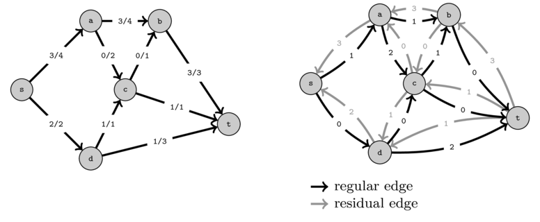
You can see that the capacities of the residual edges correspond to the amount of flow that is passing and the capacities of the original edges correspond to the original capacity minus the current flow. Thus, in the residual graph we have:
- capacity of \(residual(e) = flow(e)\)
- capacity of \(e = initialCapacity(e) - flow(e)\)
Using the residual graph, we can now very easily find new ways to push flow, we simply have to find a path of positive capacity from \(s\) to \(t\). This can be achieved using any pathfinding algorithm that we saw before.
The following figure show that the strange "path" that we used before now corresponds to a normal path in the residual graph.

If we push one unit of flow on this path we indeed obtain the same flow as before and now we get a residual graph that contains no paths from \(s\) to \(t\) of positive capacity.

It can be shown that when no more paths exist between the source and the destination in the residual graph then we have a maximum flow.
We are now going to see how we can implement this. The implementation that we will see here is not the most common or succinct but we believe that it is the one that is the closest to what we describe. We will provide later shorter implementations that are more aimed at competitive programming.
The first thing that we need is a way to represent the edges. For this we create a simple FlowEdge class containing the edge information: the origin node, the destination node, its capacity and a pointer to the residual edge.
static class FlowEdge {

    FlowEdge residual;
    int orig, dest, cap;

    public FlowEdge(int u, int v, int cap) {
        this.orig = u;
        this.dest = v;
        this.cap = cap;
    }

    public void push(int flow) {
        cap -= flow;
        residual.cap += flow;
    }

}
To represent the graph, we do the same as before except that instead of having lists of nodes we will have lists of edges. Since whenever we add an edge we need to create and add the residual edge we create a class FlowGraph with these operations.
static class ResidualGraph {

    LinkedList<FlowEdge>[] outE;
    int n;

    @SuppressWarnings("unchecked")
    public ResidualGraph(int n) {
        this.n = n;
        outE = new LinkedList[n];
        for(int u = 0; u < n; u++) {
            outE[u] = new LinkedList<>();
        }
    }

    public void connect(int u, int v, int cap) {
        FlowEdge e = new FlowEdge(u, v, cap);
        // create residual edge
        FlowEdge r = new FlowEdge(v, u, 0);
        e.residual = r;
        r.residual = e;
        outE[u].add(e);
        outE[v].add(r);
    }

}
The connect method will automatically create the residual edges. Given an edge \(e\) its residual will also have a residual edge which will correspond to the original edge \(e\). That is, \(residual(residual(e)) = e\).
We need this because when we push flow on any one of them we need to update both capacities. The following image illustrates this.
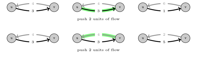
On the first case (top) we push 2 units of flow on the original edge and we reduce its capacity by 2 and increase the residual capacity by 2. The other (bottom) is analogous but we push on the residual so we decrease its capacity and increase the capacity of the original one.
All that remains is to implement the flow algorithm itself. The idea, as we discussed above, is very simple: while we can find a path \(p\) from \(s\) to \(t\) in the residual graph we push the maximum amount of flow possible on \(p\). The maximum amount of flow that we can push on a path is equal to the minimum edge capacity of that path.
static int maxflowEK(ResidualGraph g, int s, int t) {
    int maxflow = 0;
    int flow;
    while((flow = augmentFlowBFS(g, s, t)) != 0) {
        maxflow += flow;
    }
    return maxflow;
}
To find the paths we will use a BFS. The code is analogous to the one that we created before except that we adapted it to use the ResidualGraph structure.
static int augmentFlowBFS(ResidualGraph g, int s, int t) {
    // find a s-t path in g of positive capacity
    // initialize path capacities
    // pathcap[u] = capacity of the path from s to u
    int[] pathcap = new int[g.n];
    pathcap[s] = Integer.MAX_VALUE;
    // initialize parents to build the paths
    FlowEdge[] parent = new FlowEdge[g.n];
    // initialize BFS queue
    Queue<Integer> Q = new LinkedList<>();
    Q.add(s);
    // perform BFS to find a path to t
    while(!Q.isEmpty() && parent[t] == null) {
        int cur = Q.poll();
        // loop over the edges out of cur to expand the paths
        for(FlowEdge e : g.outE[cur]) {
            if(e.dest != s && e.cap > 0 && parent[e.dest] == null) {
                // we found an unvisited node e.dest
                parent[e.dest] = e;
                pathcap[e.dest] = Math.min(pathcap[cur], e.cap);
                Q.add(e.dest);
            }
        }
    }
    // check whether a path was found
    if(parent[t] == null) return 0;
    // we found a path, update the flow
    int flow = pathcap[t];
    // push the flow on the path
    int cur = t;
    while(parent[cur] != null) {
        parent[cur].push(flow);
        cur = parent[cur].orig;
    }
    return flow;
}
Note that while we perform the BFS we also keep track of the path capacity in an array pathcap. The semantics are that pathcap[u] will contain the capacity of the path from \(s\) to \(u\). Initially this will be set to \(0\) as no paths are found, except for node \(s\) which we set to \(\infty\) since the empty path from \(s\) has infinite capacity (because it has not edges).
Then whenever we find a new node \(dest\) from a node \(cur\) via and edge \((cur, dest, cap)\) we update the path capacity to reach \(dest\) to be the minimum between the capacity to reach \(cur\) and the capacity \(cap\) of the edge.
In the end we check whether a path has been found using the parent array as before. If none was found we return \(0\) because no new flow can be sent. Otherwise we push the flow on the edges of the path as explained above. This process is quite similar to the one we used to build the paths using the parents.
The runtime of this algorithm is \(O(V \cdot E^2)\). We will argue why this is the case in a later task.
The following animation gives an illustration of the maximum flow algorithm.